Verification using other libraries
### Import required libraries
import pandas as pd
import seaborn as sns
from sqlite3 import connect
import scipy.stats as stats
import statsmodels.api as sm
from statsmodels.formula.api import ols

### Required constants
DB_PATH = "../../dataset/dataset.db"
TABLE_NAME = "prj1"
<frozen importlib._bootstrap>:228: RuntimeWarning: scipy._lib.messagestream.MessageStream size changed, may indicate binary incompatibility. Expected 56 from C header, got 64 from PyObject
One way ANOVA
### Connect to sqlite3 database
connection = connect(DB_PATH)

### Create pandas dataframe for analysis
query = "SELECT * FROM " + TABLE_NAME
df = pd.read_sql(query, connection)
print(df)
      index  Less than HS    45
0         0  Less than HS  26.0
1         1  Less than HS  43.8
2         2  Less than HS  34.4
3         3  Less than HS  76.2
4         4  Less than HS   0.2
...     ...           ...   ...
1166   1166      Graduate  52.7
1167   1167      Graduate  59.8
1168   1168      Graduate  54.1
1169   1169      Graduate  39.9
1170   1170      Graduate  58.2

[1171 rows x 3 columns]
df.rename(columns = {"Less than HS": "Education Level", "45": "Salary (x1000)"}, inplace = True)
df.drop(columns = ["index"], inplace = True)

temp_frames = []
for idx, edu_lvl in enumerate(df['Education Level'].unique()):
    temp_frames.append(df[df['Education Level'] == edu_lvl].drop(columns = ['Education Level']).rename(columns = {"Salary (x1000)": edu_lvl}))

temp_df = pd.concat(temp_frames).reset_index(drop = True)

for frame in temp_frames:
    frame.fillna(frame.median(), inplace = True)

temp_df = pd.concat(temp_frames).reset_index(drop = True)
df = pd.melt(temp_df).dropna().reset_index(drop = True)
print(df)
          variable  value
0     Less than HS   26.0
1     Less than HS   43.8
2     Less than HS   34.4
3     Less than HS   76.2
4     Less than HS    0.2
...            ...    ...
1166      Graduate   52.7
1167      Graduate   59.8
1168      Graduate   54.1
1169      Graduate   39.9
1170      Graduate   58.2

[1171 rows x 2 columns]
### Visualize
temp_df.boxplot(grid = False)
<AxesSubplot:>

### ANOVA
model = ols('value ~ C(variable)', data = df).fit()
print(model.summary())
                            OLS Regression Results
==============================================================================
Dep. Variable:                  value   R-squared:                       0.015
Model:                            OLS   Adj. R-squared:                  0.012
Method:                 Least Squares   F-statistic:                     4.583
Date:                Sat, 09 Sep 2023   Prob (F-statistic):            0.00112
Time:                        18:12:27   Log-Likelihood:                -4830.6
No. Observations:                1171   AIC:                             9671.
Df Residuals:                    1166   BIC:                             9697.
Df Model:                           4
Covariance Type:            nonrobust
===============================================================================================
                                  coef    std err          t      P>|t|      [0.025      0.975]
-----------------------------------------------------------------------------------------------
Intercept                      42.1342      0.943     44.663      0.000      40.283      43.985
C(variable)[T.Graduate]         1.4936      1.531      0.976      0.329      -1.509       4.497
C(variable)[T.HS]              -2.0085      1.141     -1.760      0.079      -4.248       0.231
C(variable)[T.Jr Coll]         -1.1151      1.792     -0.622      0.534      -4.631       2.401
C(variable)[T.Less than HS]    -5.6075      1.663     -3.371      0.001      -8.871      -2.344
==============================================================================
Omnibus:                        0.362   Durbin-Watson:                   1.979
Prob(Omnibus):                  0.834   Jarque-Bera (JB):                0.431
Skew:                           0.034   Prob(JB):                        0.806
Kurtosis:                       2.935   Cond. No.                         6.26
==============================================================================

Notes:
[1] Standard Errors assume that the covariance matrix of the errors is correctly specified.
anova_table = sm.stats.anova_lm(model, typ = 2)
esq_sm = anova_table['sum_sq'][0] / (anova_table['sum_sq'][0] + anova_table['sum_sq'][1])
anova_table['EtaSq'] = [esq_sm, 'NaN']
print(anova_table)
                    sum_sq      df         F    PR(>F)    EtaSq
C(variable)    4128.063342     4.0  4.583416  0.001124  0.01548
Residual     262540.110377  1166.0       NaN       NaN      NaN
### Multiple pairwise comparisons
pair_t = model.t_test_pairwise('C(variable)')
print(pair_t.result_frame)
                             coef   std err         t     P>|t|  \
Graduate-Bachelor's      1.493552  1.530568  0.975816  0.329358
HS-Bachelor's           -2.008549  1.141209 -1.760018  0.078667
Jr Coll-Bachelor's      -1.115118  1.791994 -0.622278  0.533881
Less than HS-Bachelor's -5.607523  1.663229 -3.371468  0.000772
HS-Graduate             -3.502101  1.365669 -2.564385  0.010460
Jr Coll-Graduate        -2.608670  1.942661 -1.342833  0.179587
Less than HS-Graduate   -7.101075  1.824561 -3.891936  0.000105
Jr Coll-HS               0.893431  1.653377  0.540368  0.589047
Less than HS-HS         -3.598974  1.512860 -2.378921  0.017524
Less than HS-Jr Coll    -4.492405  2.048811 -2.192689  0.028527

                         Conf. Int. Low  Conf. Int. Upp.  pvalue-hs  reject-hs
Graduate-Bachelor's           -1.509422         4.496527   0.698372      False
HS-Bachelor's                 -4.247602         0.230505   0.336130      False
Jr Coll-Bachelor's            -4.631010         2.400775   0.782733      False
Less than HS-Bachelor's       -8.870780        -2.344266   0.006928       True
HS-Graduate                   -6.181544        -0.822658   0.080681      False
Jr Coll-Graduate              -6.420173         1.202833   0.546968      False
Less than HS-Graduate        -10.680865        -3.521285   0.001050       True
Jr Coll-HS                    -2.350495         4.137358   0.782733      False
Less than HS-HS               -6.567206        -0.630742   0.116402      False
Less than HS-Jr Coll          -8.512174        -0.472637   0.159409      False
### Tukey HSD
mc = sm.stats.multicomp.MultiComparison(df['value'], df['variable'])
mc_results = mc.tukeyhsd()
print(mc_results)
      Multiple Comparison of Means - Tukey HSD, FWER=0.05
===============================================================
  group1      group2    meandiff p-adj   lower    upper  reject
---------------------------------------------------------------
Bachelor's     Graduate   1.4936 0.8662   -2.688  5.6751  False
Bachelor's           HS  -2.0085 0.3977  -5.1264  1.1093  False
Bachelor's      Jr Coll  -1.1151 0.9715  -6.0109  3.7807  False
Bachelor's Less than HS  -5.6075 0.0069 -10.1515 -1.0635   True
  Graduate           HS  -3.5021 0.0777  -7.2332   0.229  False
  Graduate      Jr Coll  -2.6087 0.6644  -7.9161  2.6988  False
  Graduate Less than HS  -7.1011  0.001 -12.0859 -2.1163   True
        HS      Jr Coll   0.8934 0.9831  -3.6237  5.4105  False
        HS Less than HS   -3.599 0.1218  -7.7322  0.5342  False
   Jr Coll Less than HS  -4.4924 0.1831 -10.0899   1.105  False
---------------------------------------------------------------
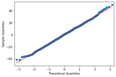
### Assumption Checks

#1) Normality using Q-Q plot
res = model.resid
fig = sm.qqplot(res, line = 's')
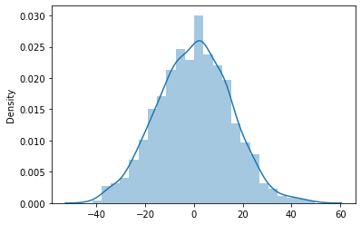
#2) Normality using Histogram Plot
sns.distplot(res, bins = 'auto', hist = True)
w, pvalue = stats.shapiro(model.resid)
print(pvalue)
0.3711097240447998


C:\Users\Jainam\miniconda3\envs\personal\lib\site-packages\seaborn\distributions.py:2619: FutureWarning: `distplot` is a deprecated function and will be removed in a future version. Please adapt your code to use either `displot` (a figure-level function with similar flexibility) or `histplot` (an axes-level function for histograms).
  warnings.warn(msg, FutureWarning)
# Homogeneity using Bartlett & Levene Tests
w, pvalue = stats.bartlett(df['value'][df['variable'] == 'Less than HS'],
                          df['value'][df['variable'] == 'HS'],
                           df['value'][df['variable'] == 'Jr Coll'],
                          df['value'][df['variable'] == "Bachelor's"],
                          df['value'][df['variable'] == 'Graduate'])

print("Bartlett's Test:\tw:{:7.4f}, pvalue:{:7.4f}".format(w, pvalue))

w, pvalue = stats.levene(temp_df['Less than HS'].dropna(), temp_df['HS'].dropna(), temp_df['Jr Coll'].dropna(), temp_df["Bachelor's"].dropna(), temp_df['Graduate'].dropna())
print("Levene's Test:\t\tw:{:7.4f}, pvalue:{:7.4f}".format(w, pvalue))
Bartlett's Test:    w:17.5776, pvalue: 0.0015
Levene's Test:      w: 5.4545, pvalue: 0.0002